透過單方向LSTM進行短時間的交通流量預測_part2.建構資料集並進行訓練_RMSE,MAE,MAPE指標模型訓練效果可視化


程式碼
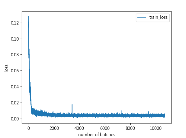
import numpy as np
import time
import math
import torch
import torch.utils.data as Data
import matplotlib.pyplot as plt
#引入sklearn現成的損失函數MSE(均方誤差),MAE(平均絕對誤差)
#MSE(均方誤差):預測值減真實值後再平分取平均
#MAE(平均絕對誤差):預測值減真實值取絕對值後再取平均
from sklearn.metrics import mean_squared_error as mse,mean_absolute_error as mae
from torch import nn
#把第一階段資料讀取處理放在另一個.py檔案引入
from trafficflow_readdata import X_train, X_test, y_train, y_test

device = torch.device("cuda:0" if torch.cuda.is_available() else "cpu")
print(device)
#透過torch.utils.data建構模型訓練需要的訓練集物件
train_dataset = Data.TensorDataset(torch.Tensor(X_train),torch.Tensor(y_train))
#將測試集轉為張量
X_test = torch.Tensor(X_test)

#用torch.utils.data建構數據產生器,按批次生成訓練數據
batch_size = 128
train_loader=Data.DataLoader(dataset=train_dataset,
                             batch_size=batch_size,
                             shuffle=True,#是否要隨機打亂數據
                             num_workers=0#是否用多process來讀數據,0就代表只有主要process去加載。
                            )
#定義mape評估指標(平均絕對百分比誤差)
def mape(y_true, y_pred):
    y_true,y_pred = np.array(y_true),np.array(y_pred)
    non_zero_index = (y_true >0)
    y_true = y_true[non_zero_index]
    y_pred = y_pred[non_zero_index]
    mape = np.abs((y_true - y_pred) / y_true)# 絕對值[(真實值-預測值)/真實值]
    mape[np.isinf(mape)] = 0
    return np.mean(mape) * 100

#設計LSTM模型類別
class MyLSTM(nn.Module):
    def __init__(self,input_size,hidden_size,layer_size,output_size):
        super(MyLSTM,self).__init__()
        self.input_size=input_size
        self.hidden_size=hidden_size
        self.layer_size=layer_size
        self.output_size=output_size
        self.lstm = nn.LSTM(input_size=input_size,
                            num_layers=layer_size,
                            hidden_size=hidden_size,
                            batch_first=True)
        self.linear = nn.Linear(self.hidden_size,self.output_size)

    def forward(self,data_points,device):
        self.h0 = torch.zeros(self.layer_size,data_points.size(0),self.hidden_size).to(device)
        self.c0 = torch.zeros(self.layer_size, data_points.size(0), self.hidden_size).to(device)
        output,(last_h,last_c) = self.lstm(data_points,(self.h0,self.c0))
        output = output[:,-1,:]
        output = self.linear(output)
        return output

input_size=1#特徵數
hidden_size=64#隱藏層單元數
layer_size=2#隱藏層數
output_size=1#輸出結果數

#建立LSTM Model物件
model = (MyLSTM(input_size=input_size,hidden_size=hidden_size,
               layer_size=layer_size,output_size=output_size)
         .to(device))
#定義損失函數為均方誤差
loss_func = nn.MSELoss().to(device)
#用自適應梯度下降做優化,learning rate:0.0001
optimizer = torch.optim.Adam(list(model.parameters()),lr=0.0001)

train_log = []
test_log = []
timestart = time.time()#開始時間
trained_batches = 0#紀錄幾個batch
for epoch in range(100):
    batchstart = time.time()#每一個batch開始的時間點
    for x,label in train_loader:
        x = x.float().to(device)#把訓練資料輸入到device中
        label = label.float().to(device)
        out = model(x,device)#獲取預測結果
        prediction = out.squeeze(-1)#去除多餘維度
        loss = loss_func(prediction,label)#計算損失函數
        optimizer.zero_grad()#梯度清零
        loss.backward()#反向傳播
        optimizer.step()#更新參數
        trained_batches += 1
        train_log.append(loss.detach().cpu().numpy().tolist())
    #測試
    X_test = X_test.float().to(device)
    pred = model(X_test,device)
    pred = pred.squeeze(-1)
    pred = pred.detach().cpu().numpy()
    #計算測試績效指標
    rmse_score = math.sqrt(mse(y_test,pred))
    mae_score = mae(y_test,pred)
    mape_score = mape(y_test,pred)
    test_log.append([rmse_score,mae_score,mape_score])
    train_batch_time = (time.time()-batchstart)
    print('epoch %d,train_loss %.6f , rmse_loss %.6f,mae_loss %.6f,mape_loss %.6f,Time used %.6f sec'
          % (epoch, loss, rmse_score, mae_score, mape_score, train_batch_time))

timesum = (time.time()-timestart)
print('總好費時長 %f sec' % (timesum))
#保存訓練模型
torch.save(model,'models/traffic_flow_model.pth')

#繪製train_loss
x = np.linspace(0,len(train_log),len(train_log))
plt.plot(x,train_log,label='train_loss',linewidth=1.5)
plt.xlabel('number of batches')
plt.ylabel('loss')
plt.legend()
plt.show()
#plt.savefig('traffic_flow_train_loss.jpg')

#繪製test_loss(RMSE)
x_test = np.linspace(0,len(test_log),len(test_log))
test_log = np.array(test_log)
plt.plot(x_test, test_log[:,0], label="test_rmse_loss", linewidth=1.5)
plt.xlabel("number of batches * 100")
plt.ylabel("loss")
plt.legend()
plt.show()
#plt.savefig('LSTMtestrmseloss.jpg')

#繪製test_loss(MAE)
x_test = np.linspace(0, len(test_log), len(test_log))
test_log = np.array(test_log)
plt.plot(x_test, test_log[:, 1], label="test_mae_loss", linewidth=1.5)
plt.xlabel("number of batches*100")
plt.ylabel("loss")
plt.legend()
plt.show()
#plt.savefig('LSTMtestrmaeloss.jpg')

#繪製test_loss(MAPE)
x_test = np.linspace(0, len(test_log), len(test_log))
test_log = np.array(test_log)
plt.plot(x_test, test_log[:, 2], label="test_mape_loss", linewidth=1.5)
plt.xlabel("number of batches*100")
plt.ylabel("loss")
plt.legend()
plt.show()
#plt.savefig('LSTMtestrmapeloss.jpg')
MyLSTM這個類別中
h0 (初始隱藏狀態)和c0 (初始單元狀態)各自都為初始化為0的張量
h0代表著每一層在處理序列數據之前的隱藏狀態的初始值。
c0 也是一個張量,形狀與 h0 相同,它保存著 LSTM 單元的初始單元狀態。負責在序列處理過程中長期保持和傳遞狀態。這一狀態允許 LSTM 跨時間步長期記憶信息,並且在適當時刻忘記無關信息。
每次當呼叫到 forward 方法時,都會初始化 h0 和 c0,並將它們作為 LSTM 層的初始狀態。
這些初始化的狀態被傳遞到 LSTM 網絡中,隨著data_points的處理,這些狀態會被更新。最終,LSTM 輸出的最後一個隱藏狀態和單元狀態(last_h 和 last_c)可用於進一步的處理或作為後續步驟的狀態。


當我們在評估回歸模型的預測效果時,常見的三個指標包括MAE(平均絕對誤差)、RMSE(均方根誤差),以及MAPE(平均絕對百分比誤差)。
這些指標各自從不同的角度評估預測值和真實值之間的差異
RMSE 均方根誤差(Root Mean Square Error)
代表模型回歸結果和真實值的平均差,是預測值與實際值之差的平方的平均值的平方根。這個指標對大的誤差給予了更大的權重,因此當模型存在較大的誤差時,RMSE會相對較高。

誤差絕對值值接球和,是預測值和實際值之間差異的絕對值的平均值。它給出了預測誤差的平均水平,並以原始數據的度量單位表示。

MAPE平均絕對百分比誤差(Mean Absolute Percentage Error)
是誤差百分比的平均值,得到的數值相對可參照性更高。
是預測值和實際值之間差異的絕對值除以實際值的平均值,通常表示為百分比。它提供了誤差相對於真實值大小的一個度量,對於衡量和比較不同規模數據的預測準確度非常有用。


留言
張貼留言