資料探勘研究與實務_Game of Thrones_A Song of Fire and Ice(Decision Tree)

冰與火之歌-預測角色是否死亡
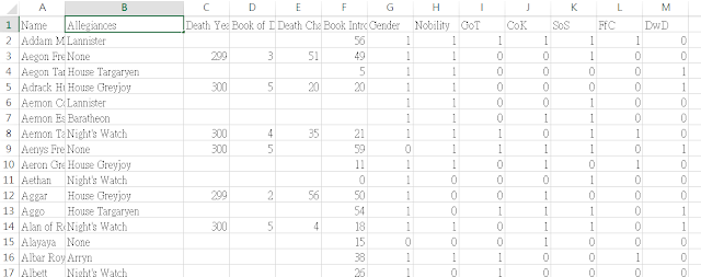
第二份資料的character-deaths.csv
其中三個欄位 Death Year , Book of Death , Death Chapter 取其中一個欄位當預測目標用即可
Step1.使用 Pandas 讀取 character-deaths.csv 資料

資料集介紹

資料集包含 917 筆和 13 個特徵。這些特徵如下:
Name: 角色的名稱
Allegiances: 角色的忠誠度或所屬派系
Death Year: 死亡年份
Book of Death: 死亡的書卷
Death Chapter: 死亡的章節
Book Intro Chapter: 角色首次出現的章節
Gender: 性別
Nobility: 貴族身份
GoT: 是否出現在 "Game of Thrones"
CoK: 是否出現在 "Clash of Kings"
SoS: 是否出現在 "Storm of Swords"
FfC: 是否出現在 "Feast for Crows"
DwD: 是否出現在 "Dance with Dragons"
Ref:
http://allendowney.blogspot.com/2015/03/bayesian-survival-analysis-for-game-of.html
將欄位的空值轉成0(代表存活),有數值的轉成1(代表死亡)
Step2-1. 用 0 替代空值。
Step2-2. 選擇 Death Year、Book of Death 或 Death Chapter 中的一個欄位作為目標變量,並將有數值的轉成 1。

將 NaN 值替換為 0,並創建了一個新的binary狀態變數 'Death',
其值為 1(如果角色已死)或 0(如果角色仍然活著或死亡狀態未知)。
Step2-3. 將 Allegiances 轉成 dummy 特徵。

Step2-4. 切分資料為訓練集(75%)和測試集(25%)。

第一階段程式
1 2 3 4 5 6 7 8 9 10 11 12 13 14 15 16 17 18 19 20 21 22 23 24 25 26 | # -*- coding: utf-8 -*- import pandas as pd from sklearn.model_selection import train_test_split data = pd.read_csv('./character-deaths.csv') # Step 2-1: Replace NaN values with 0 data.fillna(0, inplace=True) # Step 2-2: Transform 'Death Year' into binary: 1 for death and 0 for alive data['Death'] = data['Death Year'].apply(lambda x: 1 if x != 0 else 0) #data_info = data.info() #data_head = data.head() # Step 2-3: Convert 'Allegiances' into dummy variables data_dummies = pd.get_dummies(data['Allegiances'], prefix='Allegiance') data = pd.concat([data, data_dummies], axis=1) # Step 2-4: Split the data into training and test sets (75% train, 25% test) # Define predictors and target variable predictors = data.drop(columns=['Name', 'Allegiances', 'Death Year', 'Book of Death', 'Death Chapter', 'Death']) target = data['Death'] # Split the data X_train, X_test, y_train, y_test = train_test_split(predictors, target, test_size=0.25, random_state=42) |
小叮嚀: 在此所謂dummy特徵(也稱為"虛擬變數")是一種將分類變數(categorical variables)轉換為可以用於統計模型的數值型變數的方法。
給定一個分類變數,可透過創建虛擬變數來將其轉換為一組二進制(0 或 1)變數。
也就是所謂的 「one-hot encoding」

Step3.用 DecisionTreeClassifier 從 scikit-learn 來創建我們的決策樹模型。
Step4.評估模型
在訓練模型之後,就需要模型評估,計算混淆矩陣以及 Precision,Recall 和 Accuracy。
Step5.視覺化決策樹
最後第二階段程式碼
1 2 3 4 5 6 7 8 9 10 11 12 13 14 15 16 17 18 19 20 21 22 23 24 25 26 27 28 29 30 31 32 33 34 35 36 37 38 39 40 41 42 43 44 45 46 47 48 49 50 51 52 53 54 55 56 57 58 59 | # -*- coding: utf-8 -*- import pandas as pd from sklearn.model_selection import train_test_split from sklearn.tree import DecisionTreeClassifier from sklearn.metrics import confusion_matrix, precision_score, recall_score, accuracy_score import matplotlib.pyplot as plt from sklearn.tree import plot_tree data = pd.read_csv('./character-deaths.csv') # Step 2-1: Replace NaN values with 0 data.fillna(0, inplace=True) # Step 2-2: Transform 'Death Year' into binary: 1 for death and 0 for alive data['Death'] = data['Death Year'].apply(lambda x: 1 if x != 0 else 0) #data_info = data.info() #data_head = data.head() # Step 2-3: Convert 'Allegiances' into dummy variables data_dummies = pd.get_dummies(data['Allegiances'], prefix='Allegiance') data = pd.concat([data, data_dummies], axis=1) # Step 2-4: Split the data into training and test sets (75% train, 25% test) # Define predictors and target variable predictors = data.drop(columns=['Name', 'Allegiances', 'Death Year', 'Book of Death', 'Death Chapter', 'Death']) target = data['Death'] # Split the data X_train, X_test, y_train, y_test = train_test_split(predictors, target, test_size=0.25, random_state=42) # Step 3: Build the Decision Tree model tree_model = DecisionTreeClassifier(max_depth=3, random_state=42) # Limiting tree depth to 3 for visualization purposes tree_model.fit(X_train, y_train) # Step 4: Model Evaluation # Predictions y_pred = tree_model.predict(X_test) # Confusion Matrix conf_matrix = confusion_matrix(y_test, y_pred) # Precision, Recall, and Accuracy precision = precision_score(y_test, y_pred) recall = recall_score(y_test, y_pred) accuracy = accuracy_score(y_test, y_pred) # Step 5: Visualize the Decision Tree plt.figure(figsize=(12, 8)) plot_tree(tree_model, feature_names=list(predictors.columns), class_names=['Alive', 'Dead'], filled=True, rounded=True) plt.title("Decision Tree for Predicting Character Deaths") plt.show() (conf_matrix, precision, recall, accuracy) |
混淆矩陣 (Confusion Matrix)
- True Negative (TN): 130 (實際為存活,預測為存活)
- False Positive (FP): 38 (實際為存活,預測為死亡)
- False Negative (FN): 22 (實際為死亡,預測為存活)
- True Positive (TP): 40 (實際為死亡,預測為死亡)

精確度(Precision): 0.5128205128205128
表示,在模型預測為死亡的角色中,有 51.2% 確實是死亡的。
召回率 (Recall): 0.6451612903225806
表示,在所有實際死亡的角色中,模型成功預測了 64.5%。
準確度 (Accuracy): 0.7391304347826086
表示,在所有預測中,模型有 73.9% 是正確的。

視覺化決策樹

這邊調整解析度圖的尺寸另存出來看比較清晰

這棵樹根據不同特徵的分割,將樣本分到不同的分支上。
如下為此棵決策樹的視覺化呈現

這邊寫一個遞迴函數來打印各節點詳細資訊
在 print_tree_info 函數中,使用的是深度優先搜尋(Depth-First Search, DFS)的方法
來走訪決策樹。
去遞迴地打印出每個節點的資訊。
包含
samples:節點中的樣本數。
Gini:節點的Gini不純度。
class:節點中最頻繁的類別。
如果節點不是葉節點,還會打印:
分割特徵和閾值以及左右子節點的資訊
Final版本程式
1 2 3 4 5 6 7 8 9 10 11 12 13 14 15 16 17 18 19 20 21 22 23 24 25 26 27 28 29 30 31 32 33 34 35 36 37 38 39 40 41 42 43 44 45 46 47 48 49 50 51 52 53 54 55 56 57 58 59 60 61 62 63 64 65 66 67 68 69 70 71 72 73 74 75 76 77 78 79 80 81 82 83 84 85 86 | # -*- coding: utf-8 -*- import pandas as pd from sklearn.model_selection import train_test_split from sklearn.tree import DecisionTreeClassifier from sklearn.metrics import confusion_matrix, precision_score, recall_score, accuracy_score import matplotlib.pyplot as plt from sklearn.tree import plot_tree data = pd.read_csv('./character-deaths.csv') # Step 2-1: Replace NaN values with 0 data.fillna(0, inplace=True) # Step 2-2: Transform 'Death Year' into binary: 1 for death and 0 for alive data['Death'] = data['Death Year'].apply(lambda x: 1 if x != 0 else 0) #data_info = data.info() #data_head = data.head() # Step 2-3: Convert 'Allegiances' into dummy variables data_dummies = pd.get_dummies(data['Allegiances'], prefix='Allegiance') data = pd.concat([data, data_dummies], axis=1) # Step 2-4: Split the data into training and test sets (75% train, 25% test) # Define predictors and target variable predictors = data.drop(columns=['Name', 'Allegiances', 'Death Year', 'Book of Death', 'Death Chapter', 'Death']) target = data['Death'] # Split the data X_train, X_test, y_train, y_test = train_test_split(predictors, target, test_size=0.25, random_state=42) # Step 3: Build the Decision Tree model tree_model = DecisionTreeClassifier(max_depth=3, random_state=42) # Limiting tree depth to 3 for visualization purposes tree_model.fit(X_train, y_train) # Step 4: Model Evaluation # Predictions y_pred = tree_model.predict(X_test) # Confusion Matrix conf_matrix = confusion_matrix(y_test, y_pred) # Precision, Recall, and Accuracy precision = precision_score(y_test, y_pred) recall = recall_score(y_test, y_pred) accuracy = accuracy_score(y_test, y_pred) # Step 5: Visualize the Decision Tree plt.figure(figsize=(20, 12)) plot_tree(tree_model, feature_names=list(predictors.columns), class_names=['Alive', 'Dead'], filled=True, rounded=True) plt.title("Decision Tree for Predicting Character Deaths") plt.savefig("decision_tree.png", dpi=300) # Save as high-dpi PNG file plt.show() #Print and explain each node of the decision tree def print_tree_info(tree_model, feature_names, node=0, depth=0): # Print node information num_samples = tree_model.tree_.n_node_samples[node] gini = tree_model.tree_.impurity[node] class_name = tree_model.classes_[tree_model.tree_.value[node].argmax()] print(f"{' ' * depth}Node {node}: {num_samples} samples, Gini={gini:.2f}, class={class_name}") # If not a leaf node, print info for left and right children left_child = tree_model.tree_.children_left[node] right_child = tree_model.tree_.children_right[node] if left_child != right_child: # not a leaf feature = feature_names[tree_model.tree_.feature[node]] threshold = tree_model.tree_.threshold[node] print(f"{' ' * depth} Split on {feature} <= {threshold:.2f}") print_tree_info(tree_model, feature_names, left_child, depth + 1) print_tree_info(tree_model, feature_names, right_child, depth + 1) # Invoke the function to print tree info print_tree_info(tree_model, predictors.columns) (conf_matrix, precision, recall, accuracy) |
先打印當前節點(根節點)的資訊。
如果當前節點不是葉節點(即它有子節點),那就
打印用於分割的特徵和閾值。
遞迴呼叫 print_tree_info 來探訪左子節點,並增加深度計數。
在左子樹完全被探訪後,遞迴地呼叫 print_tree_info 來探訪右子節點,並增加深度計數。
Node 0: 687 samples, Gini=0.46, class=0
Split on FfC <= 0.50
Node 1: 505 samples, Gini=0.49, class=0
Split on DwD <= 0.50
Node 2: 347 samples, Gini=0.50, class=1
Split on Allegiance_None <= 0.50
Node 3: 249 samples, Gini=0.49, class=1
Node 4: 98 samples, Gini=0.47, class=0
Node 5: 158 samples, Gini=0.38, class=0
Split on Allegiance_Wildling <= 0.50
Node 6: 143 samples, Gini=0.34, class=0
Node 7: 15 samples, Gini=0.48, class=1
Node 8: 182 samples, Gini=0.25, class=0
Split on Allegiance_House Lannister <= 0.50
Node 9: 176 samples, Gini=0.24, class=0
Split on Allegiance_Night's Watch <= 0.50
Node 10: 166 samples, Gini=0.21, class=0
Node 11: 10 samples, Gini=0.48, class=0
Node 12: 6 samples, Gini=0.50, class=0
Split on Book Intro Chapter <= 3.50
Node 13: 1 samples, Gini=0.00, class=1
Node 14: 5 samples, Gini=0.48, class=0
放大從最上面看

節點 0: 這是根節點,包含所有的 687 個樣本。Gini 不純度為 0.46(不純度較高,0 表示完全純净,1 表示最不純净),最常見的類別(即這個節點的預測類別)是 0。這個節點基於特徵 FfC 進行分割,閾值為 0.50。
左側
節點 1: 包含 505 個樣本,Gini 不純度為 0.49,預測類別為 0。根據 DwD 進行分割,閾值為 0.50。
右側
節點 8: 包含 182 個樣本,Gini 不純度為 0.25,預測類別為 0。根據 Allegiance_House Lannister 進行分割,閾值為 0.50。
先往左邊Node 1後深度探討下去

節點 2: 包含 347 個樣本,Gini 不純度為 0.50,預測類別為 1。根據 Allegiance_None 進行分割,閾值為 0.50。
節點 3: 一個葉節點,包含 249 個樣本,Gini 不純度為 0.49,預測類別為 1。
節點 4: 一個葉節點,包含 98 個樣本,Gini 不純度為 0.47,預測類別為 0。
節點 5: 包含 158 個樣本,Gini 不純度為 0.38,預測類別為 0。
是根據 Allegiance_Wildling 進行分割,閾值為 0.50。
節點 6: 一個葉節點,包含 143 個樣本,Gini 不純度為 0.34,預測類別為 0。
節點 7: 一個葉節點,包含 15 個樣本,Gini 不純度為 0.48,預測類別為 1。

換右邊Node8 後深度探討下去
節點 9: 包含 176 個樣本,Gini 不純度為 0.24,預測類別為 0。
根據 Allegiance_Night's Watch 進行分割,閾值為 0.50。
節點 10: 一個葉節點,包含 166 個樣本,Gini 不純度為 0.21,預測類別為 0。
節點 11: 一個葉節點,包含 10 個樣本,Gini 不純度為 0.48,預測類別為 0。
節點 12: 包含 6 個樣本,Gini 不純度為 0.50,預測類別為 0。
根據 Book Intro Chapter 進行分割,閾值為 3.50。
節點 13: 一個葉節點,包含 1 個樣本,Gini 不純度為 0.00(完全純净),預測類別為 1。
節點 14: 一個葉節點,包含 5 個樣本,Gini 不純度為 0.48,預測類別為 0。


留言
張貼留言